Machine Learning Basics

Essentially, machine learning is a form of applied statistics with increased emphasis on the use of computers to statistically estimate complicated functions and a decreased emphasis on proving confidence intervals around these functions; therefore two central approaches are presented to statistics: frequentist estimators and Bayesian inference.

Design Matrix

One common way of describing a dataset is with design matrix.

To describe a dataset as a design matrix, it must be possible to describe each example as a vector, and each of these vectors must be the same size.

Capacity, Overfitting and Underfitting

Generalization: The ability to perform well on previously unobserved inputs is called generalization.

Difference between optimization problem and machine learning problem:

• Optimization is about minimizing "training error";
• Machine Learning's objective is to minimize "generalization error" also called "test error".

Question
How can we affect performance on the test set when we can observe only the training set?

Assumptions about how training and test set are collected are made according to statistical learning theory.

Assumptions

The training and test data are generated by a probability distribution over datasets called data-generating process.

i.i.d. assumptions:
The examples in each dataset are independent from each other, and that the training set and test set are identically distributed, drawn from the same probability distribution.

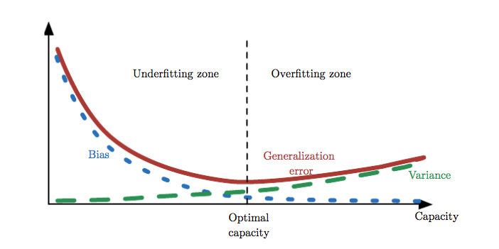
Underfitting and Overfitting

The factors determining how well a machine learning algorithm will perform are its ability to:

1. Make the training error small.
2. Make the gap between training and test error small.

We control whether a model is more likely to overfit or underfit by altering its capacity.

Capacity

Capacity is a model's ability to fit a wide variety of functions.

One way to control the capacity of a learning algorithm is by choosing its hypothesis space, i.e. the set of functions that the learning algorithm is allowed to select as being the solution.

But there are other ways to change a model's capacity.

Representational capacity of a model is achieved by finding the best function within this family of functions. in most cases however, the learning algorithm's effective capacity may be less than the representational capacity of the model family.

Occam's razor
Among competing hypotheses that explain known observations equally well, we should choose the "simplest" one.

nonparametric / parametric models

Parametric models learn a function described by a parameter vector whose size is finite and fixed before any data is observed.

Example: linear regression

Nonparametric models have no such limitation. They are theoretical abstractions that cannot be implemented in practice.

Example: nearest neighbor regression

Regularization

Idea
We can give preference to a learning algorithm, which means if both functions are eligible, one would be preferred.

Example
Modify the training criterion for linear regression to include weight decay. i.e. We prefer that weights to have smaller L2 norm. Minimizing J(w) results in a choice of weights that make a tradeoff between fitting the training data and being small, which yields solutions that have a smaller slope.

In this weight decay example, we expressed preference for linear functions defined with smaller weights explicitly. And there are many other ways of expressing preferences for different solutions, both implicitly and explicitly.

Definition of Regularization
Regularization is any modification we make to a learning algorithm that is intended to reduce its generalization error but not its training error.

note
Regularization is one of the central concerns of the field of machine learning, rivaled in its importance only by optimization.

Bias and Variance to Minimize Mean Squared Error

• Bias measures the expected deviation from the true value of the parameter.
• Variance measures deviation from the expected estimator value that any particular sampling of the data is likely to cause.

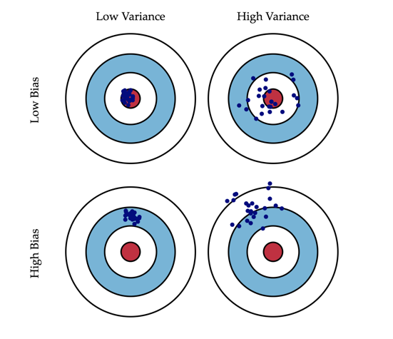
Figure credit to Understanding the Bias-Variance Trade-off. It is a wonderful blog.

Question
How do we choose between more bias and more variance?

• The most common way to negotiate this trade-off is to use cross-validation.
• Alternatively, we can compare mean squared error (MSE) of the estimators.

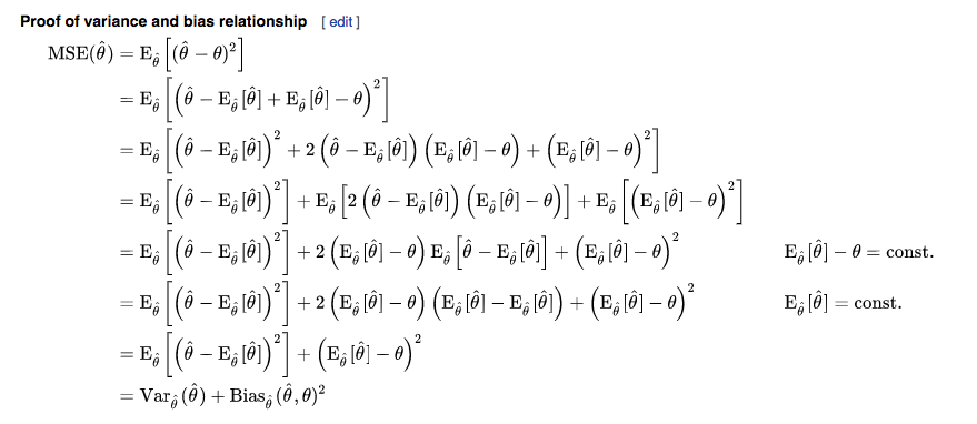
Mean Squared Error (MSE)

The MSE measures the overall expected deviation -- in a squared error sense -- between the estimator and the true value of the parameter theta.

The relationship between bias and variance is tightly linked to the machine learning concepts of capacity, underfitting and overfitting.

Consistency

We wish as the number of data points m in our dataset increases, our point estimators converge to the true value of the corresponding parameters.

The symbol plim indicates convergence in probability.

Maximum Likelihood Estimation

Maximum likelihood is the most common principle behind modeling estimators.

The problem formulates like following,

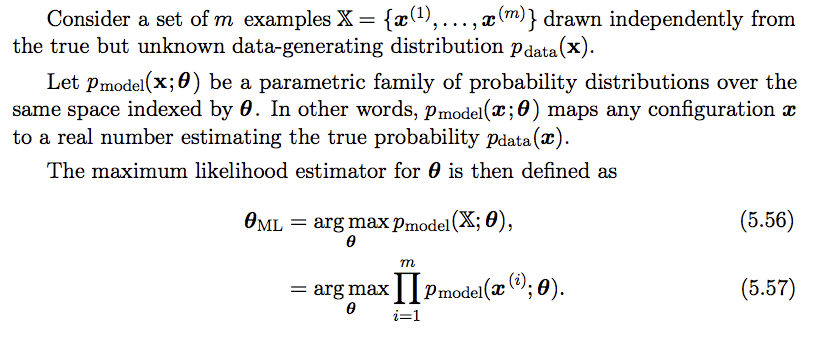
The formulation has one shortcome that the product form is prone to numerical underflow. Therefore we take logarithm of the likelihood which does not change its arg max operation.

Interpretation of Maximum Likelihood Estimation

One way is to view it as minimizing the dissimilarity between the empirical distribution p_data, defined by the training set and the model distribution, with the degree of dissimilarity between the two measured by the KL divergence. The KL divergence is given by,

Note that the term on the left is a function only of the data-generating process, not the model which means we only consider minimizing the KL divergence,

Interpretation
Maximum likelihood is our attempt to make the model distribution match the empirical distribution not the true data-generating distribution which we have no direct access to.

Properties of Maximum Likelihood

consistency and efficiency

Consistency

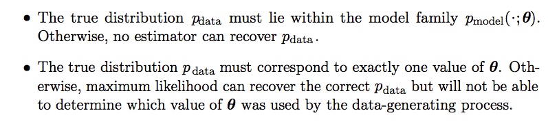
Under appropriate conditions, the maximum likelihood estimator has the property of consistency, i.e. as the number of training examples approaches infinity, the maximum likelihood estimate of a parameter converges to the true value of the parameter. These conditions are,

(Statistical) Efficiency

One consistent estimator may obtain lower generalization error for a fixed number of samples m, or equivalently may require fewer examples to obtain a fixed level of generalization error.